Epistemic Status: This is not my speciality within ML and I present mostly speculative intuitions rather than experimentally verified facts and mathematically valid conjectures. Nevertheless, it captures my current thinking and intuitions about the phenomenon of ‘grokking’ in neural networks and of generalization in overparametrized networks more generally.
Recently, I saw a fascinating paper by Alethea Power of OpenAI describing a phenomenon which she calls ‘grokking’ in neural networks. The core idea is that if you train a neural network for many, many, many epochs after the training loss has gone to zero, such that it appears you are doing nothing more than massively overfitting, at some point there is instead a sudden phase change towards a low validation loss – i.e. the network has somehow (suddenly!) learnt to generalize even though training error has been at zero for many many epochs. The killer figure from the paper is presented below:
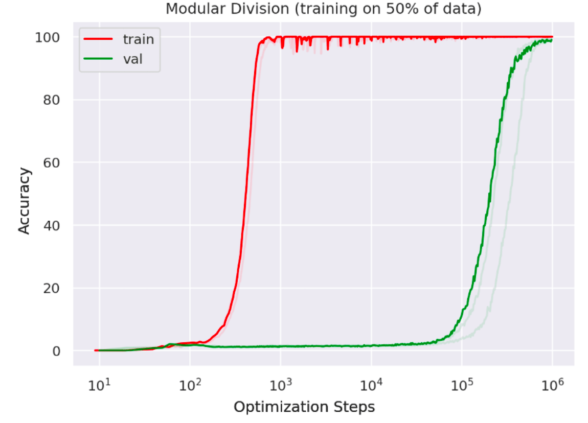
What is happening here? Whatever it is it certainly cannot be explained by standard statistical learning theory which would predict a dismal future of eternal overfitting.
To really understand what is going on, we need to think about what is happening during training in overparametrized networks in terms of the optimal set. The optimal set, which I’ll denote \(\mathcal{O}\), is the set of all parameter values which result in 0 training loss on the dataset. Specifically, to understand grokking, we need to understand what the optimal set looks like as networks become increasingly overparametrized.
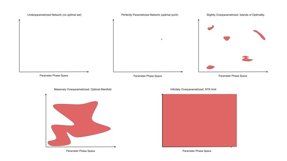
For an underparametrized network, the optimal set is empty. No parameter settings can exactly reproduce all the data in the dataset. In the more familiar terms of sets of linear equations, we have more constraints than variables so there is no exact solution. This is the domain of standard statistical learning theory and in this regime we can derive bounds on the degree of overfitting and hence bound the generalization loss. Intuitively we can think of networks of this regime as not having the representational capacity to memorize the data so instead they are forced to find the ‘best fit line’ – i.e. to find some reasonable interpolation between the data points. Because of insufficient representational capacity, this interpolation cannot vary arbitrarily in between datapoints but must take some simple form and this results in a smooth function which gets pretty close to most datapoints and does not vary wildly in between them – in essence, the network is forced to generalize (under the assumption that the true data is drawn from some smooth manifold underlying around the datapoints).
Then, as representational capacity increases, we reach the threshold of perfectly parametrized models where there is exactly one optimal point. Our number of equations exactly matches our number of unknowns so there is a single ‘correct’ solution. The optimal set holds only a single point. Now, as statistical theory tells us, since we have just enough representational capacity to perfectly memorize the training data, it also has the freedom to vary arbitrarily away from the datapoints, and often because of the artificial nature of this solution (it is really just fitting noise), it will often do so. The optimal point exists but it may be very very far from the optimal solution in terms of generalization loss. We have entered the realm of overfitting.
But the story does not end here. We can continue adding parameters and representational capacity into the network and obtain overparametrized networks. We now have more variables than constraints and so we have an infinity of solutions. The optimal set grows in number and becomes a volume. In the case of linear equations, we know exactly what happens with the optimal set – it becomes a linear hyperplane of dimension \(E - U\) where \(E\) is the number of equations and \(U\) is the number of unknowns. However, for deep networks in practice, the geometry of the optimal set will be much more complex than that of the linear system of equations, and currently seems poorly understood. However, understanding and quantitatively describing this geometry will be key to understanding generalization in overparametrized networks and in ultimately deriving improved learning algorithms to grok faster and more robustly.
As the network moves past its perfectly parametrized state and slowly becomes overparametrized, what happens to the optimal set? To begin, we get scattered points and ultimately ‘islands’ of optimality forming as occasional and distributed parameter combinations becomes optimal (of course technically there are an infinite amount of such islands and maybe some infinite ‘channels’ connecting them representing redundant of nuisance parameter dimensions, but crucially the volume of the optimal set is still incredibly small compared to the non-optimal set). We now turn to the other side of the equation: given such an island archipelago, what will stochastic gradient descent (SGD) do during training? It will be initialized somewhere, walk towards an island close to where it started, fall into the island (almost certainly a bad one in terms of validation loss) and then get stuck. SGD will explore the small volume of the island but it cannot get out because it is surrounded by vast oceans of suboptimality and the distance to the next island is too great for SGD to ever ‘tunnel’ across the surrounding suboptimality due to gradient noise. The network is stuck. It will not grok or ever exhibit good generalization performance. It will just stay overfit indefinitely. In one sense the network failed because it was overparametrized, but in another because it was not overparametrized enough.
So what happens if we add more parameters? The volume of the optimal set grows relative to the total vollume of parameter space. The islands of optimality grow closeer and closer together and eventually begin to merge, creating large-scale connected optimal surfaces or optimal manifolds in parameter space. If the number of parameters grows large enough, tending to infinity, then the optimal set becomes everywhere such that it lies infintesimally close to all points in the parameter space. This is exactly what happens in the NTK limit of infinite neural network width where, as the number of parameters (width) tends to infinity, the change in weights between the networks at initialization and after training tends to 0. This vanishing difference allows you to mathematically express the trained network as a first order Taylor expansion around the networks initialization from which we can derive the usual properties of the NTK and occurs because the network can reach optimality with an infintesimal perturbation of its parameters – the optimal manifold is infinitely close.
The key thing is that with a large enough degree of overparametrization we begin to get a notion of a coherent ‘optimal manifold’. Now, we need to think about what does SGD now do in the presence of such a manifold. At first it just gets initialized at some points and descends towards the manifold, hitting it at some mostly random point. Then, if training is continued when it is on the manifold, it will essentially perform a random walk on the manifold, driven by gradient noise, and slowly move across it due to diffusion.
If we stop training as soon as we hit the optimal manifold or before, as is commonly done in practice, then we simply get the generalization error of the random point where SGD hits the optimal manifold. But, if we keep SGD running, eventually over time, due to its random walk behaviour, it will gradually diffuse through and slowly explore the optimal manifold until, potentially much much later, it stumbles upon a region with much better generalization performance – i.e. ‘grokking’.
In short this is my intuition for what grokking is:
1.) A sufficiently overparametrized neural network possesses a coherent and spatially contiguous optimal manifold.
2.) SGD first falls towards and hits the manifold (standard training) and once it is on the optimal manifold performs a diffusive random walk across it.
3.) The optimal manifold contains regions of greater or lesser generalization performance, with most regions representing useless overfitting but some regions where the parameter space matches the ‘true function’ in some sense where the network can obtain high generalization performance.
4.) Ran long enough, SGD will eventually drift into these ‘generalizing regions’ and the network will appear to show ‘grokking’.
The Bayesian Interpretation as MCMC
But in ML we have seen something very like this play out before in the theory of Markov Chain Monte Carlo methods. For a fantastic introduction to the intuitions I’m trying to convey here see this paper. In short, MCMC methods provide a way to sample from a distribution (usually a Bayesian posterior) which we cannot compute directly and does not need to be normalized. The idea is simply to run a Markov Chain with an equilibrium distribution equal to the desired posterior, initialize it somewhere, wait a while for the chain to reach equilibrium, and then take samples from the chain as samples from the unknown posterior we were wanting to compute.
Theoretically, this process can be described in terms of a ‘typical set’ of a high dimensional probability distribution. The typical set is a relatively small volume (compared to total volume spanned by the distribution) where almost all the probability mass concentrates. The typical MCMC chain will converge to the typical set (burn-in phase) and then, if the geometry of the typical set is not pathological, explore across it, generating high value posterior samples.
If we step back a little, this process sounds identical to grokking scenario described earlier with SGD and the optimal set. We simply have swap out the MCMC chain -> SGD and the typical set -> the optimal set. What is more, we know this is more than a superficial anoalogy, but is instead mathematically justified. We know that SGD itself can be considered a MCMC algorithm.
But if SGD is the markov chain, what posterior distribution is represented by the optimal set? Again this is obvious. The ‘optimal set’ is simply the posterior distribution over the weights given the data $p(w | D)$. Why? Note first that by Bayes theorem we have that: \(\begin{align} p(w | D) = \frac{p(D | w) p(w)}{p(D)} \end{align}\) Since we are performing MCMC we don’t need to care about the normalization constant \(p(D)\) so we can just write this as \(p(w | D) \propto p(D | w) p(w)\). Next we assume we have no prior over the weights, or a uniform prior, which allows us to ignore the prior term and just write \(p( w | D) \propto p(D | w)\). But for the overparametrized case \(p(D | w)\) is a strange object. For all parameter settings which lead to incorrect predictions of the data \(p(w | D)\) is obviously 0 since we have the capability of making correct predictions, and for all parameter settings which lead to perfect prediction we have that \(p(D | w) \propto 1\). However, since we have no reason to prefer at this point any particular parameter setting to any other, we see that \(p(D | w)\), and hence \(p(w |D)\) is simply a uniform distribution over the optimal set. So when SGD is diffusing over and exploring the optimal set, we can interpret this as SGD being a MCMC sampler, ‘sampling’ values from the posterior over the weights.
The Weight Decay Prior
So far we have ignored the role of the prior and assumed a uniform distribution over weight values, but what if we don’t assume this. Specifically, the grokking paper found that a crucial technique to improve grokking times was weight decay and specifically weight decay towards the origin (0) and not weight decay towards the initialization. Luckily, this result is straightforward to understand a-priori. It is well known that weight decay can be interpreted in Bayesian terms as a zero-mean Gaussian prior for each weight. To see this, consider SGD with weight decay, \(\begin{align} \frac{dW_{i,j}}{dt} = - \eta \frac{\partial L}{\partial W_{i,j}} - \alpha W_{i,j} \end{align}\) Where \(\eta\) is a learning rate for the gradient step and \(\alpha\) is the weight decay coefficient. We can express the weight decay update as the gradient of a log probability \(- \alpha W_{i,j} = \frac{\partial \log p(w_{i,j})}{\partial w_{i,j}}\) where \(p(w_{i,j}) = \mathcal{N}(w; 0, \sigma^2)\) where \(\alpha = \frac{1}{\sigma^2}\) so that the strength of the weight decay is directly related to the precision of the prior, which makes sense. Essentially, what weight decay is doing is improving performance by switching SGD from traversing the likelihood posterior but a posterior affected by a zero-mean prior. If we assume that the best generalizing regions are likely located close to the origin, then this effectively substantially reduces the optimal manifold volume that SGD has to diffuse through to find the generalizing region and therefore dramatically cuts the time to grok.
Sampling and the Geometry of the Optimal Set
Now that we have described the connection between MCMC and grokking via the optimal set, there is a key insight from the MCMC theory literature which we could utilize to potentially massively speed up grokking time. Namely, that if we understand the geometry of the optimal set, then we can design sampling schemes that can explore much more efficiently and rapidly than SGD. Secondly, if we can understand the relationship between the geometry of the optimal set and the number of parameters and network architectures, then it may be possible to design architectures which lead to nicer geometries and do not lead to optimal manifolds with geometric pathologies such as regions of extremely high curvature, which tend to impede MCMC sampling. This would lead to network architectures which are ‘designed to grok’, in some sense.
However, the connection to MCMC will likely lead to immediate gains by applying more efficient samplers developed for MCMC to neural network training, or at least grokking once the typical set has been reached. Stochastic Langevin sampling (what SGD technically is) is known to be a very poor and inefficient smapler due to its random walk nature. Other methods such as Hamiltonian MCMC tend to explore the optimal set much more efficiently than SGD will, and could hence potentially substantially speed up grokking. Moreover, if we know about the curvature of the optimal set, we could also apply Riemannian MCMC sampling methods which explicitly take into account the curvature maintaining an estimate of the metric and moving accordingly in the space. This could again lead to more efficient sampling over SGD which implicitly assumes a space of unit variance and do very poorly in other regimes.
Beyond this, a proper mathematical grasp on the geometry of the optimal set will allow us to answer fascinating theoretical questions like:
1.) What is the optimal range of overparametrization needed to show grokking – is there eventually a tipping point where additional overparametrization hurts. The evidence that NTK infinite-width models tend to generalize worse than finite width models suggests that there is. Finding and understanding this ‘sweet spot’ will be very fruitful.
2.) What is the minimum number of parameters or optimal set size needed to show grokking – i.e. maintain a connected volume that SGD can diffuse across while also containing the ‘true’ parameter settings needed for generalization.
3.) What does this mean and how does it interact with the effect of number of parameters on performance discovered by the scaling laws papers.
4.) Which network architectures and datasets lead to well-behaved non pathological optimal sets which can easily be explored and hence ‘grokked’.
5.) Where in the optimal set does the ‘true’ generalizing solution tend to lie – can we design better priors for this than \(\mathcal{N}(w; 0, \sigma^2)\)?
Why Weight Decay? A Solomonoff Induction Perspective
Although we have ‘explained’ the effectiveness of weight decay as it being a Gaussian prior on the weights around 0, this explanation actually leaves much to be explained. Specifically, why should we expect weights of magnitude close to 0 to generalize better than weights far from 0?
Although much needs to be worked out formally, the intuition for an answer can be seen by looking at Solomonoff induction. This is an ‘optimal’ method for any inference problem, but is incomputable. As such it describes the limit case of optimal inference. Essentially, Solomonoff induction performs Bayesian inference with the hypothesis set being that of all programs. The data we are given is some string of bits such as 0100110011110101… and the hypothesis class is the set of all programs, encoded somehow (details don’t matter) into Turing machines, that output some string of bits. Given this setup, we then perform exact Bayesian inference. All programs which fail to predict a certain bit get chucked out – set to probability 0 – so the size of the hypothesis space halves with each bit – i.e. we gain 1 bit of information per bit, thus achieving 100% efficiency. Nevertheless, our hypothesis class is an infinite space of all possible programs, so we need to deal with that somehow.
The solution is to set a prior distribution over programs. This is the Solomonoff prior which downweights programs exponentially in their Kolmogorov complexity – i.e. ‘longer’ programs receive exponentially decreased weight in the prior. The reason for this is that the number of possible programs grows exponentially with the program length, and so that as length increases there are exponentially more possible ‘distractor’ programs which produce the correct bit string by chance than that actually compute the ‘true’ function encoded in the bit string. For instance, suppose we have the bit string “11111111111 … 1111”, there is the ‘true’ program which is something like “print N 1s” and then there are exponentially many distractor programs which do irrelevant things and then just happen to print “11111111111 … 1111”. The key is that the true program should be much shorter, in Kolmogorov complexity terms, than the distractor programs, and so will receive exponentially greater weight in Solomonoff induction. The Solomonoff prior, then, formalizes the principle of Occams razor that simpler hypotheses are to be preferred.
A similar argument applies to the magnitude of the weights of an overparametrized network. Intuitively, for a given dataset with some general scale, we naively expect the ‘true program’ that generated the dataset to contain weights roughly within that scale, usually small. If your data is within \([0,1]\) it seems very unlikely that the program which generated this data contains weights of magnitude \(10^{200}\). However, as with programs, the ‘volume’ of weight space that can be used to fit the data increases polynomially with weight magnitude – approximately \(M^W\) where \(M\) is the largest weight magnitude and \(W\) is the cardinality of the weight space. This means that to encode an Occams razor principle, we should enforce this polynomial decay with a prior. Indeed, it seems that the quadratic penalty of weight decay is actually less severe than the combinatorics would suggest and perhaps instead we should use an exponential or high-order polynomial weight decay penalty.