Predictive Coding as Backprop and Natural Gradients

This post explores some lesser known and recently discovered connections between predictive coding algorithms and the backpropagation of error algorithm in machine learning, as well as natural gradient methods. The material on natural gradients is novel to this post (as far as I know). Prerequisites are a general understanding of variational inference and linear algebra, as well as ideally some basic knowledge of predictive coding. For really good tutorial introductions to predictive coding I would recommend this one (for a basic walkthrough) and this one (for the full mathematical construction).

Predictive Coding (and the more general designation predictive processing) is an influential theory in theoretical neuroscience which purports to offer a general theory of cortical function. Predictive coding has also made strides towards a more popular audience, where it has been explained in various blog posts as well as in more popular books like Andy Clark’s Surfing Uncertainty, which provides a fantastic introduction and intuition pump for the theory.

The high-level story is that the brain is fundamentally in the business of minimizing prediction errors – i.e. the difference between what you expect to happen and what actually happens. By updating the internal parameters (synaptic weights) of your brain to minimize this difference you eventually get better at predicting the external world – i.e. you learn about the world. Action can also be explained in this story by saying that another way of minimizing prediction error is to change the external world itself to bring it in line with your predictions. You can change the world through actions, so you can derive the optimal action as the one which brings the world most in line with your prediction

A key element of this predictive processing story is that the brain is hierarchical and composed of multiple layers, each of which is attempting to minimize its own prediction errors. Crucially, each layer sends its predictions to the layer below, and attempts to predict the activity at that layer. Any discrepancy between the top-down prediction of the superordinate layer and the actually realized activity of the subordinate layer is seen as a prediction error to be minimized by the higher layer. Importantly, real external sensations enter at the bottom of this hierarchy so that the first layer tries to minimize the prediction error of its predictions compared to the real input. As it does so, it will necessarily change away from the top-down predictions conveyed by the second layer, so the second layer will experience prediction error, and so forth. In this way, unpredicted elements of the external world ripple up the hierarchy until they reach a level at which they can be explained. Interestingly, this framework can be shown mathematically to be implementing hierarchical variational Bayesian inference under certain assumptions (Gaussian variational posterior and generative model). If the brain followed this scheme, it would mean that the brain was fundamentally implementing an approximate form of Bayesian inference, which if true would be a fantastic insight and provide a general organizing principle for understanding brain function.

It is important to separate out distinct levels of predictive processing/predictive coding theory. First there is the very high level idea of predictive processing which states that the brain implements bayesian inference, specifically approximate variational bayesian inference, and it achieves this by minimizing prediction errors. The second theory is a low-level mathematical theory which allows you to write down the exact dynamics of the cortical neurons according to this model. This is where the idea of prediction error minimization arises. However, it is important to note that recognizable prediction errors arise from very specific assumptions about the nature of the approximate posterior and the generative models used in bayesian inference. The brain could still be performing variational inference, but with a different parametrisation of the variational density, and it would not give rise to prediction error minimization.

The high level story says that the “parameters” of the brain “change to minimize “prediction error”, but have been very vague about what the parameters are and what this “change” is that occurs. To make this into a real theory, we need to make these notions mathematically precise.

Let us suppose we are working with leaky integrate and fire neurons, so that each neuron entails the function \(y = f(\theta x)\) where y is the output activity, f is a nonlinear activation function, \(\theta\) is a synaptic weight and \(x\) is a vector of all inputs. We can concatenate an array of neurons together to obtain the vector equation \(\mathbf{y} = f(\Theta \mathbf{x})\). From here on out we will only ever be talking about the vector equations so, for simplicity, we will write them with the same notation as the single neuron equation. Let us write down a model with multiple hiearchical layers of neurons, with top down predictions and bottom up prediction errors. The top-down prediction reaching level \(x_i\) is simply, \(\begin{align} \hat{x_i} = f(\theta x_{i+1}) \end{align}\) We define the prediction errors \(\epsilon_i\) to be simply the difference between the top down predictions reaching a layer and the activities at that layer, \(\begin{align} \epsilon_i = x_i - \hat{x_i} \end{align}\)

From this we can define learning rules that minimize the prediction errors for both the activities of each layer \(x_i\) and the synaptic weights between layers \(\theta_i\), \(\begin{align} &\frac{dx_i}{dt} = -\epsilon_i + \epsilon_{i-1} \frac{\partial f(\theta x_i)}{\partial x_i} \theta_i^T \\ &\frac{d\theta_i}{dt} = -\epsilon_i \frac{\partial f(\theta_i x_i)}{d\theta_i}x_i^T \end{align}\)

This means that the dynamics of the activations at any layer are affected by the prediction error at the current layer plus the prediction error at the layer below mapped upwards through the transpose of the top-down weights. This is why we speak of predictions errors being propagated “upwards” in this framework. Importantly, all of these rules are fundamentally Hebbian (meaning they only require the multiplication of pre and post synaptic activity) and require only local connectivity. This means that this algorithm can be straightforwardly implemented in the brain, and people have put forward realistic neural process theories which propose ways in which this could be done.

These rules also have a much deeper interpretation in terms of variational bayesian inference. First, consider the objective function which, for reasons that will become clear soon, we denote $\mathcal{F}$, that must be implicitly being optimised to produce the dynamics above. With a little mathematical imagination, we can work this out to be

Or simply the sum of squared prediction errors at each layer. If we squint at this a little we can see that a squared prediction error is also the log probability density of a gaussian with a variance of 1, plus a constant of \(\ln 2 \pi\). If we extend this a little further, we can understand this objective as a variational free energy functional between a gaussian variational posterior and a gaussian generative model

With this objective, we can interpret the predictive coding dynamics as performing a gradient descent on this variational free energy, and thus performing variational inference. Since we have a hierarchy of layers \(x_{0:L}\), we can write the variational density and generative model as \(q(x) = \prod_{i=0}^L\) and \(p(x,\theta) = p(x_L)\prod_{i=0}^L p(x_i \vert x_{i+1}; \theta)\), which gives us hierarchical Bayesian inference.

This gaussian assumption also gives us an additional set of parameters to play with – the precisions (or inverse variances) \(\Sigma^{-1}\) of the gaussian distribution, which we have previously taken to be 1 (or the identity matrix in the multivariate case). However, if we work back through all of the equations without this assumption of the variance being identity, we can obtain the following dynamics, \(\begin{align} &\frac{dx_i}{dt} = -\epsilon_i \Sigma^{-1}_i+ \epsilon_{i-1} \Sigma^{-1}_{i-1} \frac{\partial f(\theta x_i)}{\partial x_i} \theta_i^T \\ &\frac{d\theta_i}{dt} = -\epsilon_i \Sigma^{-1}_i \frac{\partial f(\theta_i x_i)}{d\theta_i}x_i^T \end{align}\)

as well as also the ability to derive the dynamics for the precisions themselves, \(\begin{align} \frac{d \Sigma^{-1}_i}{dt} = \Sigma^{-1}_i - \Sigma^{-1}_i \epsilon_i \epsilon_i^T {\Sigma^{-1}_i}^T \end{align}\)

These precisions play an important role in the more detailed and nuanced description of the theory, and can be thought of as modulatory factors that weigh the relative importance of one set of prediction errors against another. For instance, they could weigh relative importance of top-down vs bottom up processing, or at a finer level of detail, the importance of some parts of an image compared to other parts for classification. At this fine-grained level of detail, we can think of precisions as parametrising attention. You brain receives an extremely large amount of sensory input every second, and only attends to a small fraction of that. Mathematically this selection mechanism of attention could be thoughts of as applying a low precision weighting to the majority of the input and a high precision weighting to those parts of the input that are attended to. This means we can look at the precision matrices as a kind of attentional saliency matrix.

This idea of precision as parametrising attention plays a significant role in the theory. A significant part of Andy’s book, for instance, deals with the possible effect on processing of different levels of precision, and the phenomenology of various psychiatric or other cognitive disorders such as autism and schizophrenia can be described in terms of aberrant precision weighting.

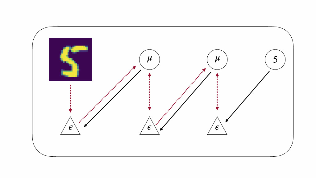
So far, we have thought about predictive coding as a kind of autoencoder (a neural network which is trained to reconstruct its own inputs). However, we can also think about predictive coding as a generative model for supervised learning where, at the top level of the hierarchy, a label is presented and the task of the predictive coding model is to generate sensory data consistent with the label. In your brain this underlies your ability to imagine sensory (for instance visual) features of an object (say “a cat”) given only a verbal or otherwise high level description. This conditional generative capability of predictive coding networks has been evaluated in the literature. This is all still currently in line with the story above about predictions flowing down and prediction errors flowing upwards.

Now for the twist. Suppose we flip the order of the network so that the label sits at the ‘bottom’ of the network and the visual input (say an image) sits at the ‘top’. We can think of this as the network is trying to predict the “sensory input” the label from the “prior knowledge” the image. Now this sounds like, and mathematically is a standard classification problem addressed in standard machine learning where you have a deep neural network trying to predict a label (cat or no cat) from an image.

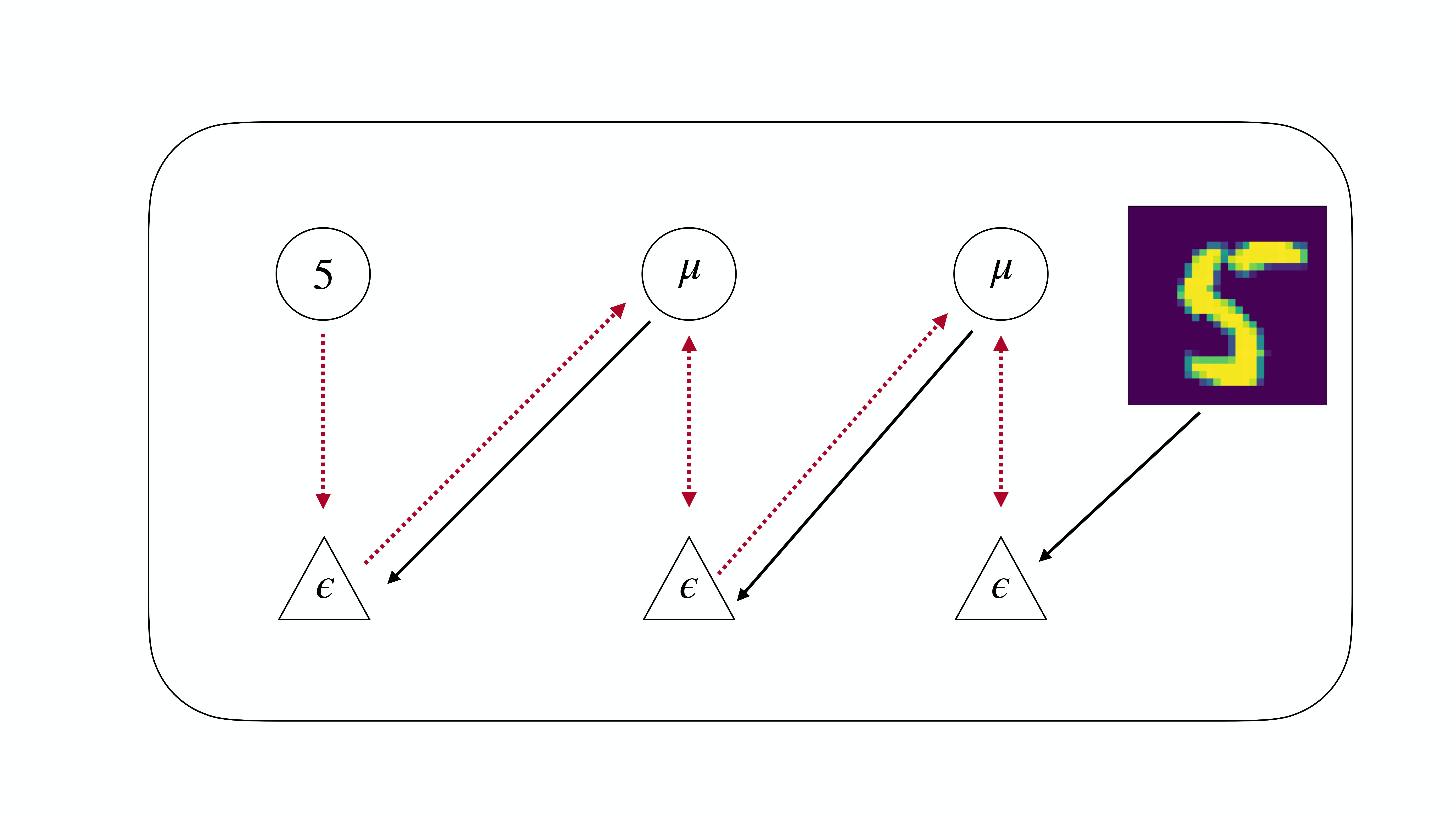
To make this analogy more clear, we also flip the names of prediction errors and predictions so that we now have ascending “predictions” and descending “prediction errors”. We can think of the ascending “predictions” as like the forward pass in a deep neural network. But what are the descending “prediction errors”? Amazingly, in 2017 Whittington and Bogacz showed that if the network is allowed to settle into an equilibrium where the “prediction errors” are minimized, the equilibrium value of the prediction errors is exactly equal to the gradients computed by backpropagation. This “reverse” predictive coding is simply backprop, and is exactly equivalent to training a MLP network with a standard machine learning library like PyTorch or Tensorflow. In my recent paper, I showed that this equivalence can be extended not just to multi-layer perceptrons as shown by Whittington and Bogacz, but to any arbitrary computation graph. This means that you can use predictive coding to, in theory, train any modern machine learning architecture. Predictive coding is, in fact, a fully general automatic differentiation algorithm. I demonstrate this by training predictive coding CNNs and LSTMs, but it can be extended to even more modern architectures like GRUs, ResNets and, crucially, Transformers.

To get across the full impact of this, let me say it again. We have a neuroscientific theory of cortical function which originated in the late 90s and was developed in the early 2000s, before modern machine learning. This theory proposes biologically plausible learning rules and update which could in theory be implemented in the brain, to the extent that there have been worked out cortical microcircuits which can implement predictive coding. Moreover, predictive coding has been validated against a substantial amount of empirical neurophysiological data, and has been utilised to understand the symptomology of neurological and psychiatric disorders. The same theory, when run in reverse, turns out to be identical with modern machine learning, and crucially implements the backpropagation of error algorithm which is currently the only scalable optimisation algorithm known which is able to efficiently optimize extremely deep neural networks.

Isn’t that amazing? It’s perhaps the closest bridge we currently have to understanding how biological intelligence implemented in brains and artificial intelligence implemented by deep neural networks relate to one another. Moreover, if it is fundamentally true that the brain implements something like predictive coding, and therefore something like backprop, this has huge implications in general. It would mean that the current paradigm of machine learning is sufficient to replicate much of the core functionality of the brain. This would have significant implications for projected AI timelines.

This equivalence between reverse predictive coding and backpropagation also implies a number of other fascinating things. We know that predictive coding is a hierarchical bayesian variational inference algorithm. Therefore this means that we can understand backpropagation in this manner too. Specifically backpropagation arises as a hierarchical variational inference algorithm which infers the value of each node of the computational graph under gaussian assumptions. This close link between optimsiation algorithms and inference is fascinating and may be really fruitful in understanding what is really going on at a deep level in these systems.

The second fascinating thing is how to understand the precisions of the original predictive coding in light of backpropagation. To obtain the equivalency to backpropagation we must set the precisions all to 1 (or the identity matrix in the multivariate case), which means that they have no effect. But imagine if they did have an effect. What this would mean is that it is possible to have a kind of uncertainty aware backprop, where the influence of various inputs or nodes in the computation graph can be modulated depending on its inherent noise, and so have less influence on the overall outcome. This could provide a highly flexible and robust stochastic backpropagation algorithm which can natively handle uncertainties across the computational graph. The precisions = I assumption crucially encodes the i.i.d assumption which is that all data is equally important and equally variable for the network. This is true in the standard machine learning settings where we have a given dataset and simply want to optimize against this dataset but is not true in the real world where for a biological agent there is a vast amount of ‘distractor’ information at any point which must simply be ignored. This also fits in with the attention story of precision from before, but applied to learning instead of perception. I.e. that we only select some information as important for learning and only update based on that information. This is not necessarily the same (but could be in practice) as the information we explicitly attend to. Figuring out whether the brain implements learning-attention as well as perception-attention, and whether these two attention types can be dissacociated would be really fascinating as a neuroscientific study.

From the machine learning perspective, it is also possible that by explicitly constructing our optimisation algorithms such as backprop to have some measure of attention to filter out distractor stimuli may improve performance and add robustness in more realistic environments. For an initial taster of this we showcase our final result (which to my knowledge is novel to this blog post), which is that if we do perform backpropagation in which we learn and optimize the precisions \(\Sigma^{-1}\), then this is equivalent to a natural gradient descent on the internal optimisation of the \(v\)s. This is important because natural gradients are in some sense the “correct” way to do gradient descent which takes into account the true geometry of the space. Crucially, the information contained within the precision matrices which takes into account the uncertainty of the input has a deep relationship to the geometry of the optimisation landscape.

Natural gradients are a simple idea arising from information geometry. See here and here for detailed and deep descriptions. If we consider the standard gradient descent update as \(\begin{align} x^{t+1} = x^t + \eta \frac{\partial L}{\partial x} \end{align}\)

Where \(x\) is the variable being optimized, \(\eta\) is some learning rate, and \(L\) is the loss function. The natural gradient update is simply \(\begin{align} x^{t+1} = x^t + \eta \mathcal{G}(x) \frac{\partial L}{\partial x} \end{align}\)

where we multiply the gradient by the prefactor \(\mathcal{G}\). This prefactor is a very special quantity called the Fisher information, which is a deep information theoretic quantity. The Fisher information mathematically is the simply the variance of the score function (gradient of the log density) or, alternatively, the curvature of the log density. In this equation it serves the purpose of a metric in differential geometry and effectively scales the space by the curvature of the log likelihood function ¹.

The intuition behind this is that if you first consider the standard gradient descent equation, it updates each direction the same amount, paying no heed to how much the loss function actually changes in that direction. However, this is clearly suboptimal. If the loss function is changing rapidly in a certain direction, then you really only want to go a small distance in that direction, since the real gradient is changing rapidly under your feet – and you are effectively only equipped with a local linearisation of the true gradient (at your start point). On the other hand, if the loss function in another direction is extremely flat, you want to take a large step in that direction, as your gradient vector is likely to remain very stable for quite a large distance so it is a waste to take a bunch of tiny little steps and recompute the gradient each time. The Fisher Information metric (or the curvature of the log density) proves to be the ideal quantity that lets you compute how much the gradient of the loss function is changing at every point. By multiplying the gradient vector by the Fisher Information precisely, you embed this information into the optimisation process so that you only move a small distance in directions of rapid fluctuations of the loss, and a large distance where change is slow. In theory, this lets you choose a larger learning rate, since you are automatically slowed down in regions of rapid change, and don’t have to rely on the learning rate to do this. Natural gradients may also arguably improve convergence speed and robustness.

When precisions are included we can show that the relevant update rules for the activity units \(v\) and the weight matrices \(\theta\) are simply, where \(\mathcal{\tilde{F}}\) is the free energy without precisions: \(\begin{align*} v^{t+1} &= v^t + \eta \Sigma^{-1} \frac{\partial \mathcal{\tilde{F}}}{\partial v_i} \\ \theta^{t+1} &= \theta^t + \eta \Sigma^{-1} \frac{\partial \mathcal{\tilde{F}}}{\partial \theta_i} \end{align*}\)

From this we can see the direct analogy to natural gradients. If the Fisher information is simply the precision then we have that predictive coding with precisions is implementing natural gradients. We next show that equality is the case for the activity units, and thus the gradient descent on the activities becomes a natural gradient descent when precisions are taken into account. We can see that the fisher information of the activity units is the precision as follows: \(\begin{align*} \mathcal{G}[v_i] &= \mathbb{E}[\frac{\partial^2}{\partial v_i^2}\mathcal{F}] \\ &= \mathbb{E}[\frac{\partial^2}{\partial v_i^2}(v_i - f(\theta_i v_{i-1}))^T\Sigma^{-1}_i (v_i - f(\theta_i v_{i-1}))] \\ &= \mathbb{E}[\frac{\partial^2}{\partial v_i^2} v_i^T \Sigma^{-1}_i v_i ] \\ &= \mathbb{E}[ \Sigma^{-1}_i] \\ &= \Sigma^{-1}_i \end{align*}\)

Now, this is a fascinating result because it shows that there is a deep connection between the modulatory aspects of attention, the uncertainty inherent and encoded in each stage of the computation graph, and the fundamental information-geometric properties of the free energy manifold.

In the linear case, the Hessian of the free energy with respect to the weights is also straightforward, as we show below. In this case the natural fisher information is equal to the precision multiplied by the variance of the presynaptic activities, which could also be computed locally by the brain (albeit requiring integration over time). This means that in theory this could be computable and utilized in the brain. \(\begin{align*} \mathcal{G}[\theta_i] &= \mathbb{E}[\frac{\partial^2}{\partial \theta_i^2}\mathcal{F}] \\ &= \mathbb{E}[\frac{\partial^2}{\partial \theta_i^2}(v_i - \theta_i v_{i-1})^T\Sigma^{-1}_i (v_i - \theta_i v_{i-1})] \\ &= \mathbb{E}[\frac{\partial^2}{\partial \theta_i^2}v_{i-1}^T \theta_i^T \Sigma^{-1}_i v_{i-1} \theta_i ] \\ &= \mathbb{E}[ v_{i-1}^T \Sigma^{-1}_i v_{i-1} ]\\ &= \Sigma^{-1}\mathbb{E}[v_{i-1}v_{i-1}^T] \end{align*}\)

However, in the nonlinear case the expression becomes considerably more complex. This means that it is unlikely that the full nonlinear Fisher Information with respect to the weights can be computed locally by neurons. However, it is possible that the linear version could actually be a good approximation of the full nonlinear Fisher, so that we could consider predictive coding with precisions to be implementing some kind of approximate natural gradient descent in weight-space. Figuring out to what extent this approximation holds, if it holds at all, would be a really fascinating further direction here.

(1) The use of the Fisher Information as a metric in differential geometry is integral to the field of information geometry which uses it to define a metric on a manifold of the parameters of (exponential family) probability distributions.